The Data Collection Handbook · Part IV. Running It at Scale

Chapter 13. Operating at Scale

David Martin Riveros · Published August 22, 2026

A fleet I ran once locked up with every worker alive and answering its health check. The intake was accepting jobs. And no customer got data, because one large retail site had slowed to a crawl, every worker in the pool was holding one of its half-finished jobs, and every other customer's work sat in line behind them. A whole fleet, one slow source, zero deliveries. I spent an hour restarting things in the wrong order before I understood there was nothing to fix. The system was doing exactly what I had built. I had built one line.

Growing from one collector to a fleet changes the collectors less than you would expect. What changes is the wiring between them, and the wiring is where fleets die. So this chapter is about wiring: queues that keep one slow source from stalling everyone, concurrency treated as a promise instead of an accident, rescue for work that falls asleep, a scheduler that starves no one, and the discipline for the nights when all of it fails anyway. In the middle sits a sizing question with a trap in it, and the experiment walks into the trap on purpose, with the meter running.

Queues between stages

A queue is a humble thing: a list of work waiting its turn, kept somewhere that survives a crash. That humility is the point. The night I described had no queues worth the name, just workers calling sources and each other directly, so the slowness of one site traveled through the whole system like tension through a rope.

A fleet that survives is built as stages with queues between them. Five stages cover almost every collection operation I have seen. Accept takes the customer's submission and records it. Schedule decides what runs next and under which limits. Collect fetches from the sources. Process parses and validates what came back, the work of Chapters 7 and 8. Deliver writes the result where the customer receives it and proves it landed, the work of Chapter 12. Each stage reads jobs from a queue, does its one thing, and writes to the next queue. No stage calls another. The queue is the only thing they share.

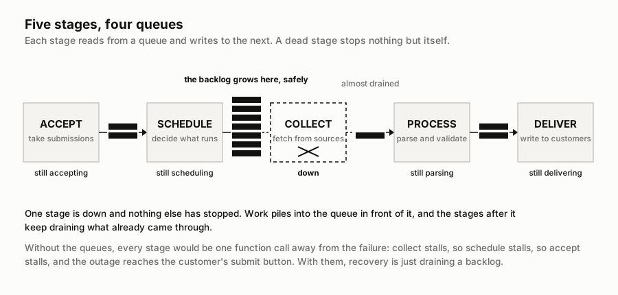
Now replay my bad night in this design. The slow site drags the collect stage, and only the collect stage. Submissions still land. Scheduling still happens. Parsed results still flow to customers whose data was already fetched. The backlog piles up in one queue, in one visible place, where you can measure it, alarm on it, and drain it when the site recovers. An outage becomes a number going up instead of a company going dark.

One word makes the design hold: backpressure. When a queue grows past a set depth, the stage feeding it slows down or starts answering not yet. The pile-up travels backward, stage by stage, until it reaches the edge of the system, where the customer is told queued instead of getting a fast acceptance that means nothing. A system without backpressure accepts work it cannot do and hides the truth in the middle of the pipeline. With it, the truth surfaces at the intake, which is the only place anyone can act on it.

Concurrency is a promise

Two limits govern how hard a fleet pulls, and confusing them is the commonest operations mistake I know. Concurrency, how many jobs run at the same moment, feels like one knob, and it is actually two.

The first is the per-source ceiling: how many requests you allow against one source at once. Chapter 2 argued that the load you put on one source belongs to the source, sized to what it can absorb without noticing you; a simultaneous-request ceiling is that rule translated into fleet vocabulary, and Chapter 6 taught the reflexes, backing off and breaking the circuit, for when you got it wrong. At fleet scale the ceiling stops being a politeness and becomes an entry in a table: this source, at most this many at once, enforced by the scheduler no matter how much work is waiting or how many workers are free.

The second is global capacity: how many workers you pay to exist. That number belongs to your budget and to the promise you made customers about wait times. It has nothing to do with what any source tolerates.

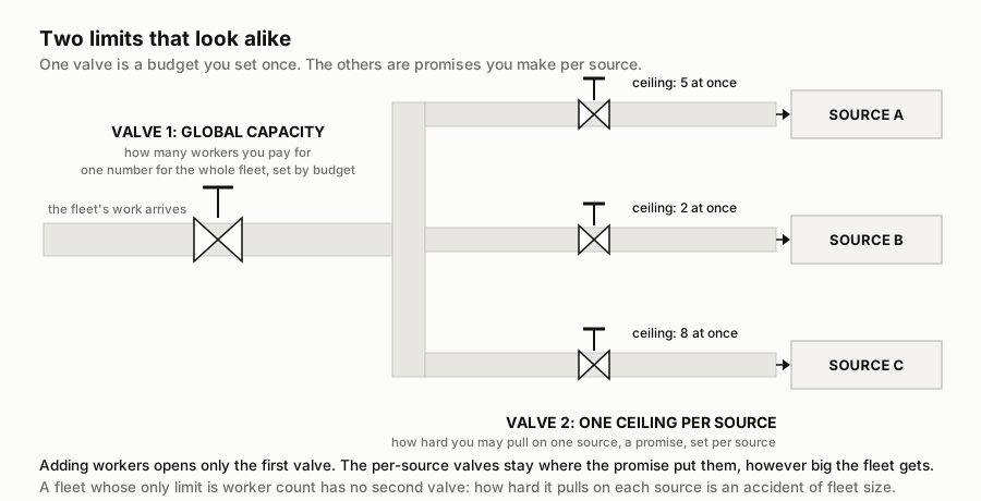
Keep the two valves separate and boring things stay boring. You can double the fleet for a growing customer and no source feels a thing, because the ceilings did not move. You can tighten one source's ceiling after a rough week without touching capacity anyone else uses. But if your only limit is worker count, then every scaling decision silently changes how hard you hit every source, and the day you add twenty workers for one customer is the day a different customer's source starts blocking you. On my bad night the coupling ran the other way, one source's slowness absorbing the fleet, and the missing piece was that same per-source table.

Nothing sleeps forever

Workers die mid-job. A machine gets reclaimed or a process runs out of memory; sometimes a network partition swallows a whole box. None of that is exceptional at fleet scale; with dozens of workers it is a normal week. The design question is what happens to the job the dead worker was holding, because the naive answer is: nothing, forever. The records say running, no process is actually running it, and the customer waits. Operators call these zombie jobs, and a fleet without a plan for them leaks work continuously.

The plan has three parts. First, taking a job is a lease rather than an ownership transfer: the job disappears from the queue for a limited time, sometimes called a visibility timeout, rather than being deleted. Second, the worker holding a lease sends heartbeats, small I am alive signals on a fixed rhythm, and each heartbeat extends the lease. Third, silence expires it. Miss a few beats and the job simply reappears in the queue, where the next free worker picks it up as if nothing happened.

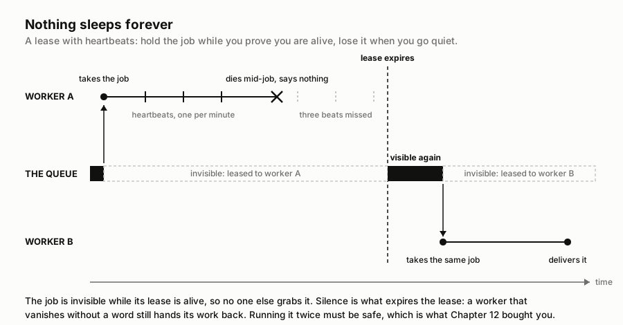
Notice what the design refuses to depend on: the worker saying goodbye. A crash announces nothing. Recovery keyed to error messages misses the deaths that matter, so recovery is keyed to the absence of a signal instead. Silence is the one thing a dead worker reliably produces.

There is a catch, and it is why this chapter comes after Chapter 12. A lease that expired because a worker was slow, not dead, means two workers now run the same job. You will tune timeouts to make that rare. You cannot make it impossible, and a distributed fleet that promises exactly-once execution is lying to itself. The real contract is at least once, which is only safe because Chapter 12 made delivery idempotent: running the same job twice lands the same files under the same names, and nothing downstream doubles. Rescue without idempotency is a duplicate generator.

One habit turns all this into something you can trust: run the rescue sweep on a schedule, every few minutes, as a boring background chore. A recovery path that only executes during disasters is untested by definition. Mine runs all day and finds nothing, and the finding nothing is the test.

Scheduling the fleet

With the stages decoupled and the zombies handled, someone still decides which waiting job runs next. The default answer, first in, first out, has a fairness problem that shows up the first week you have two customers. One submits a 10,000-job catalog backfill at 9:00. Another submits 3 urgent jobs at 9:01. Under first in, first out, those 3 jobs wait behind all 10,000, and your smallest customer just learned that your biggest customer owns the fleet.

The fix is to stop pretending there is one line. Give each customer their own queue and serve them round robin, one turn each in a circle, or in weighted shares if contracts differ. Inside a customer's queue, let priorities exist: a small urgent refresh should overtake that same customer's own background backfill. And push heavy recurring work into off-peak windows, the source's quiet hours, which Chapter 2 already argued is kinder to the source; it also happens to be when the fleet has slack.

Scheduling cannot create capacity. The experiment below held its scheduling fixed at plain first in, first out, and its final limit says why that was fine: priorities and fairness reallocate waiting between jobs; they do not reduce the total. When the whole fleet is behind, no ordering saves you.

How many workers does the promise really take

The last knob is the size of the fleet itself, and it hides the most expensive mistake in this chapter. The promise at stake is the one queues make visible: how long a job waits before it starts. Customers feel that wait directly, so it ends up in contracts as a service level agreement, an SLA. The experiment uses a common shape: 95% of jobs start within 5 minutes of submission.

The scenario's numeric assumptions sit in one editable file (example/data/params.json), and its two distribution shapes, geometric batch sizes and exponential service times, live in run.py: jobs arrive at 30 an hour on average, each takes 10 minutes of work on average, with individual jobs running shorter or longer the way real jobs do, so customers offer the fleet 5 hours of work every hour. A worker costs $65 a month, the scenario's assumed price for a small always-on cloud machine. The whole thing is seeded and offline; python run.py reproduces every number and both charts.

How many workers? There is a formula, and it is a century old. A. K. Erlang, a Danish engineer at the Copenhagen Telephone Company, worked out in 1917 how many operators an exchange needs so that callers rarely wait. Callers dial one at a time. The queueing mathematics named after him, Erlang C, answers our question, provided jobs arrive the way callers do, smoothly, one at a time at random moments, and run long or short the way calls do. For this load it says 8 workers, with a p95 wait of 4.0 minutes, inside the promise. The p95 wait is the wait the unluckiest 1 job in 20 experiences. And the formula is no relic: the experiment's discrete-event simulation, a program that replays the queue arrival by arrival, measures 3.8 minutes at those same 8 workers under smooth arrivals. A hundred years on, Erlang is still right about the world he described.

The trap is that fleets do not live in that world. Nobody submits jobs one at a time. A customer presses go on a category refresh and a dozen jobs land in the same second. So the experiment runs the same average load a second way: batches land at random moments, each carrying a random number of jobs averaging 12. Statisticians call the arrival pattern compound Poisson. Same 30 jobs an hour. Same 5 hours of offered work. Only the clumping changes.

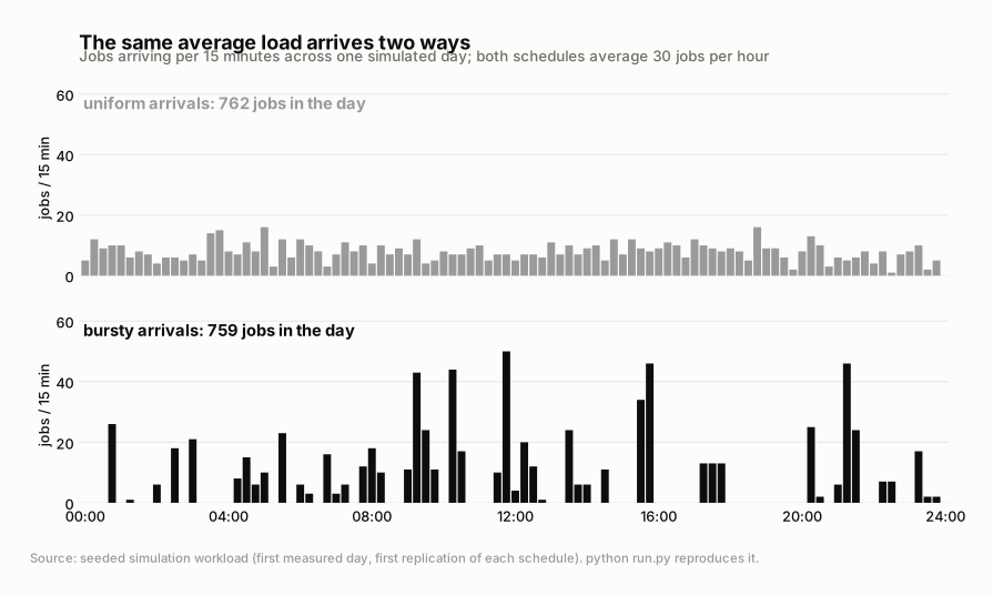
Under the batched arrivals, the promise takes 31 workers, holding a p95 of 4.7 minutes with 95.3% of jobs inside the promise (202,287 of 212,352 across ten simulated months). The formula's answer of 8 undershoots by a factor of about 4, at the same average load, on the number customers feel.

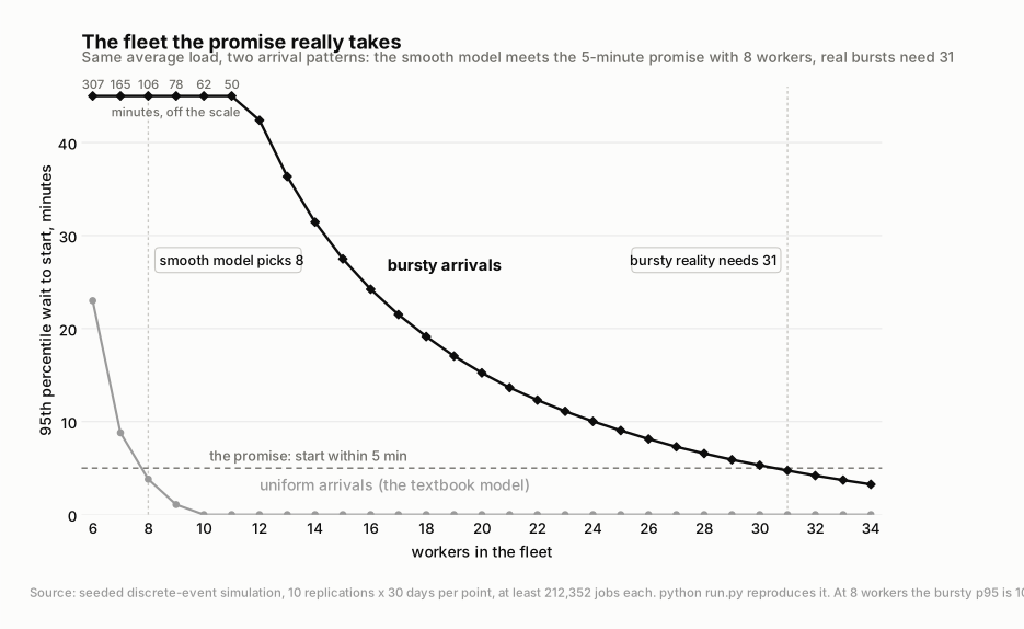
Run the 8-worker fleet the formula recommends under the real arrivals and the failure is not subtle. The p95 wait is 106.4 minutes against the 5 promised, 21 times the promise. Of 212,352 jobs, 149,679 miss it, 70.5% of everything submitted. And while that happens, the utilization dashboard reads 62%. Utilization, the share of time the average worker is busy, is exactly the number an average-load dashboard shows you, and at 62% it looks like a healthy shop with room to spare. Chapter 10 showed a green dashboard hiding rotting data. The same thing happens here on the operations side: a green dashboard hiding a broken promise.

The mechanism is a job's position inside its own clump. With batches averaging 12, some batches run long, and 10,767 of the 212,352 jobs, 5.1%, arrive 35 or more jobs deep in their own submission. Starting a job that deep within 5 minutes means clearing the 34 ahead of it within 5 minutes, and a busy worker frees up about once every 10 minutes. No plausible service speed clears a clump that fast. The only thing that does is workers already standing idle when the batch lands.

This is why the right-sized fleet looks absurd on every chart a finance review will ever produce. At 31 workers, utilization is 16%. At a random moment, about 5 of the 31 are busy. Those 26 idle workers are the promise, held in reserve for the next batch. And the promise has a price: at $65 per worker the formula's fleet costs $520 a month and the fleet that keeps the promise $2,015, a gap of $1,495 for identical average throughput. When you quote an SLA, that gap is what the SLA costs to be true, and Chapter 11's cost-per-record arithmetic should be charged with it.

That price will be challenged, so arm whoever defends it. In this sweep, cutting the fleet from 31 workers to 20 saves $715 a month and drops the share inside the promise from 95.3% to 82.3%, which is 2,756 more late jobs a month averaged over the ten simulated months, roughly four newly late jobs for every dollar saved. When a budget review calls the reserve idle, do not argue philosophy. Put the late-job count next to the savings and let the review own both numbers.

The brief's hypothesis, written before the code ran, was that burstiness, not average load, sets the fleet size, and that the smooth-arrivals model undersizes badly at the promise customers feel. The run confirmed both, 8 against 31. One finding I did not predict: the damage is not confined to the tail. At the 8-worker fleet the median wait is 18.4 minutes, so half of all jobs break the 5-minute promise. I had expected a story about unlucky jobs at the 95th percentile. The data says the typical job fails, and half of everything a customer submits arrives late.

The numbers come with three limits. The factor of about 4 belongs to this scenario; heavier batch tails push it up, capped batches pull it down, and the right move is to rerun the sweep with your own measured arrivals, which is what the parameters file is for. Elastic capacity, starting workers when a batch lands, shrinks the $1,495 rather than the worker count, because the burst still has to be served by capacity that exists at burst time. And even 31 is a pooled answer: single simulated months range from 3.7 to 5.9 minutes at the p95, so a contract read strictly month by month takes 33.

Read those limits again as a price list, because two of them are contract clauses. The arrival shape is the expensive one: both fleets serve the same 30 jobs an hour, so the $1,495 buys the customer's habit of landing a dozen jobs in the same second. A customer who agrees to pace a big refresh is cheaper to serve, which is a discount you can offer or a burst fee you can charge. The measurement window is the cheap one: reading the promise strictly month by month costs two extra workers, $130 a month. I price both on purpose now, instead of discovering them in a bad quarter.

Incident discipline

The bad night comes anyway. Queues, ceilings, leases, and a fleet sized for real arrivals make it rarer; nothing makes it never. Operations that survive their incidents agreed the steps in advance; the ones that skip that get defined by their incidents. And 3 a.m. is a bad time to invent process.

Start with a severity ladder, written down while everyone is calm. A SEV1 means a customer promise is being broken right now: deliveries failing, or wrong data flowing. A SEV2 means the promise is at risk but holding, a backlog growing faster than it drains. A SEV3 is internal pain nobody outside would notice. The ladder matters because at 3 a.m. everything feels like a SEV1, and the severity written next to each alarm is what stands between a team and treating them all the same.

Then the first three moves, in order. First, stop the bleeding: mitigate before you diagnose. Pause intake for the affected source so backpressure does its job, flip to the fallback method from Chapter 3's waterfall, let Chapter 6's breaker stay open. Understanding why can wait an hour; the meter of broken promises cannot. Second, one owner, speaking out loud: a single person runs the incident and posts short factual updates on a fixed rhythm, including to affected customers. Chapter 12 made the case that customers verify you anyway; a customer who hears about the incident from you trusts the next delivery more, not less. Third, preserve the evidence before you heal the patient. Snapshot the queue depths and capture the logs before anything restarts, and write down the times, because a restart erases the evidence the write-up will need.

Tomorrow's job is the write-up, and the rule that matters there is that it names the mechanism rather than a culprit. That is mechanics as much as kindness: an operator who expects punishment stops reporting near-misses, and near-misses are the cheapest early-warning signal an operation ever gets; Chapter 10 priced what late detection costs. The write-up has three parts, a timeline, a mechanism, and a change: some ceiling, timeout, alarm, or runbook line that is different now. My one-line test for whether an incident is closed: point to the thing that changed. If nothing changed, the incident is still open, however long ago the outage ended.

Who notices first

I rank a data operation by one question: when something breaks, who notices first? The answers form a ladder, and every operation I have seen sits somewhere on it. On the first rung, a person watches it: dashboards and a morning scroll. Detection is whoever happens to be looking. On the second, the system pages a person: Chapter 10's alarms wired to queue depth, zombie counts, and the promise itself, the p95 start wait measured per customer on the same clock the contract uses. On the third, the system handles its own routine failures, the zombie sweeps and open breakers and backpressure of this chapter, and pages a human only for what it lost. On the fourth, the system proves its promises: delivery verified at the destination as Chapter 12 demanded, the start-time promise reported from measurement, the fleet resized when measured burstiness drifts from the assumption it was sized for.

One demotion protects the second rung: take utilization off the service page entirely. In the experiment it read 62% while seven of every ten jobs ran late, and 16% while the promise held, so it measured cost correctly both times and never measured service at all. My rule for the weekly review: the first fleet number anyone sees is the p95 start wait per customer, and utilization lives in the budget review, where it tells the truth.

Most operations I meet live on rung two and describe themselves as rung four. The tell is always the same: the promises are stated, never measured.