The Data Collection Handbook · Part IV. Running It at Scale

Chapter 11. Cost Engineering

David Martin Riveros · Published August 20, 2026

I have sat through many versions of the same budget review. A slide reports that the collection stack runs at a tenth of a cent per request, the room relaxes, and the meeting moves on to something that looks riskier. The number on the slide is usually true. It is also the most flattering number the operation could have chosen to report, because nobody in that room is buying requests. The customer is buying records that arrive, and the economics of this trade live in the distance between those two things.

So this chapter is about one number: cost per successfully delivered record. Take every dollar the operation spends and divide it by the count of rows that actually reached the customer. The definition sounds obvious. Its bite is in what it does with failure. A failed attempt is a cost with no denominator, spend that cannot carry itself, so its price has nowhere to go except into the records that did arrive. Count failure that way and several habits that look normal in this industry start looking off.

The only number that matters

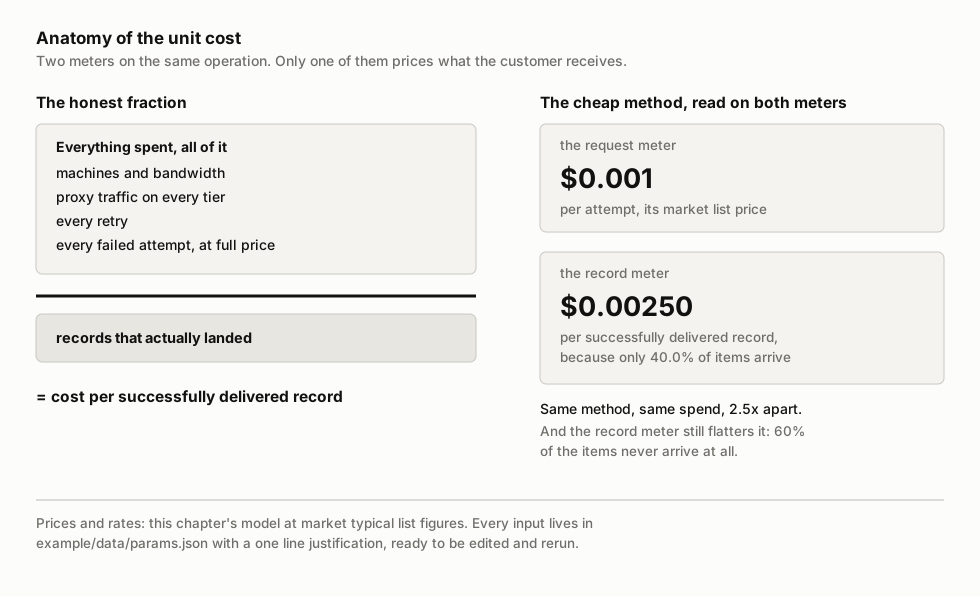
Cost per request divides spend by everything you tried, and trying is the one thing your successes and your failures have in common. Trying is the biggest divisor you can pick, which is why the number comes out so small, and that is how it ends up on slides. Cost per delivered record divides the same spend by what landed, and nothing else about the arithmetic changes.

The gap between the two meters is wide. Take the cheapest method in this chapter's model, a plain HTTP fetch from datacenter addresses at $0.001 per attempt, the model's market list figure. On a defended site the model gives it a 40% success rate, and the delivered-record meter turns a tenth of a cent into $0.00250 per delivered record. It was always this expensive; the request meter could not see it. Even that second meter is still flattering this method, because 60% of the items never arrive at all, and a unit cost says nothing about the rows it walked away from.

Anatomy of the unit cost

What belongs in the numerator is all of it. The machines that run the collectors. The bandwidth. The proxy traffic on every tier, which Chapter 4 taught you to buy deliberately rather than by reflex. Every retry, because Chapter 6's backoff discipline spends real attempts. Every failed attempt, at full price. And the people, which polite cost models omit and serious ones put first: Chapter 1's build-vs-buy model found engineering at 92 percent of the in-house bill at its breakeven volume, and nothing in this chapter repeals that finding.

What this chapter's model prices is deliberately narrower: the attempt costs, what you pay each time you press the button. People costs move slowly, and Chapter 1 already modeled them. Attempt costs respond to routing decisions you can change this week, which makes them the lever worth isolating. The model uses three methods at market typical list figures. A plain datacenter fetch at $0.001 per attempt, succeeding on 40% of items. The same fetch through residential addresses at $0.010, succeeding on 75%. And a rendering or unblocker style product, the managed services that fetch a hard page for you at a per-page price, at $0.050, succeeding on 98%. Every one of those assumptions lives in a small shipped file (example/data/params.json) with a one line justification beside it. Disagree with any of them, edit the file, rerun the model.

Run the delivered-record meter over the premium method alone and you get the first lesson in unit anatomy. At $0.050 per attempt and a 98% success rate, the cost per delivered record is $0.05102. The missing 2% of attempts did not vanish from the books: they were paid for, delivered nothing, and reappeared inside the price of everything that landed. That mechanism is failure amortization. It sits inside every unit cost, and it grows fast as success rates fall.

The waterfall as an economic instrument

Chapter 3 built the waterfall as an architecture: find every door into a source, order the doors by price, send every item to the cheapest first, and let only the failures fall through to the next one. There the argument was machine time and the numbers were illustrative. Here the waterfall becomes the main instrument of cost engineering, and the numbers come from a model you can rerun and argue with.

Walk a thousand items through the model's three tiers, taking the list rates at face value for a moment and rounding to whole items. The cheap tier tries everything and delivers 400. The 600 leftovers fall to the mid tier, advertised at 75%, so it should deliver 450 and pass 150 on. The premium tier, at its advertised 98%, rescues 147 of those and leaves 3 undelivered. Total spend: $1.00 on the cheap tier, $6.00 on the mid, $7.50 on the premium, $14.50 for 997 delivered records. That is $0.01454 per delivered record, against $0.05102 for sending everything through premium. A 3.51x saving, and the waterfall even delivers more, 99.7% of items against 98.0%, because three chances at an item beat one. One definition, since this is the number the mix produces: the blended cost is the average cost per delivered record across all tiers together, and it is the only unit cost a mixed operation actually has. On those numbers you would sign today.

Do not sign yet.

The success rates in that arithmetic are brochure rates, each method's score when the whole population of items is thrown at it, and the arithmetic assumed, without saying so, that they were independent, as if every attempt were a fresh coin flip. In production they are not. An item that failed the cheap method is usually a hard item, a defended endpoint, an odd template, a page behind aggressive protection, and hard items fail the next method more often too. Difficulty travels with the item rather than the attempt. The mid tier never sees the population its brochure was measured on; it sees the cheap tier's rejects. How much that one fact moves the answer is exactly what this chapter's experiment measures.

What correlation does to the promise

I wrote the hypothesis in the brief before the model ran. It said: a tuned waterfall cuts blended cost several-fold against premium-only, and correlated difficulty erodes the naive estimate enough to matter, which is why the mix must be tuned from measured per-tier success rates rather than brochure numbers. Two clauses. The run judged both.

The model gives every item a hidden difficulty drawn from a bell curve and lets each method's chance of success fall as difficulty rises. One dial sets how much of success lives in the item against the individual attempt. At one end, every attempt is an independent coin flip, the brochure world above. At the other, difficulty is a strict ladder: an item too hard for premium is too hard for every method beneath it. And the uncomfortable part: at every level of the dial, each method is re-calibrated so its population-wide success rate still matches its brochure, so correlation leaves every brochure true and changes only what the leftovers look like. The run evaluates all 15 orderings and subsets of the three methods at 11 correlation levels, computes exact answers by numeric integration, and cross-checks its headline cell with a seeded 200,000-item simulation. Everything is offline; python run.py reproduces every number in this chapter and the chart below.

Its tables print a moderate correlation level, one that lands the mid method at a measured 63.8% on the cheap method's leftovers, nearer the strict ladder than independence. At that level, the same thousand items come out differently.

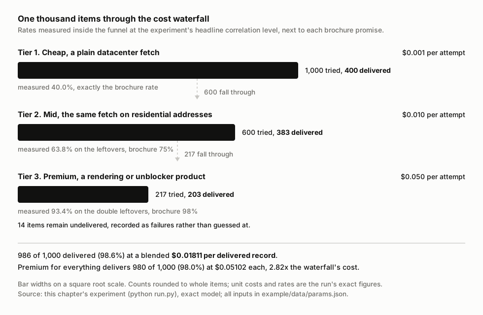
The cheap tier still delivers its 400; it goes first, so the brochure rate is the measured rate. The mid tier delivers 383 of its 600, a measured 63.8% against the advertised 75%. The premium tier rescues 203 of the final 217, a measured 93.4% against the advertised 98%. Fourteen items end the day as recorded failures. Delivery lands at 98.6% instead of the promised 99.7%, and the blended cost lands at $0.01811 per delivered record instead of the promised $0.01454.

Set the two funnels side by side and take the two clauses in turn. The saving survives: $0.01811 against premium-only's $0.05102 is 2.82x, and no correlation level in the sweep pushes the ratio below 2.56x, the strict-ladder worst case, where the waterfall costs $0.01990 per delivered record. The erosion is real too, and material: the true unit cost ran 25% above the naive plan, and coverage came in under the promise, 99.7% promised against 98.6% real. The three chances mostly stopped being three chances, because the leftovers are the hard items every tier struggles with. Both clauses held, the first at nearly threefold even in the worst case. And notice what the brochures did through all of this: nothing wrong. Every method held its advertised rate on the full population at every correlation level, and the plan built on those rates still missed. The numbers stayed true and still misled, which is harder to catch than a vendor fudging.

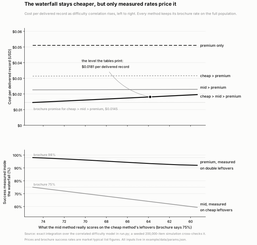
The sweep behind the chart adds a finding I did not put in the brief, and it is the one I use most. The erosion has a floor. As correlation rises from coin flips to a strict ladder, the waterfall's cost climbs from $0.01454 to $0.01990 and stops there, because once difficulty is a perfect ladder there is nothing left to correlate. Cheapest-first remains the winning ordering at every level of the sweep, and the waterfall never comes close to losing to premium-only. Correlation re-prices the decision without ever reversing it. So you can choose a waterfall without knowing your correlation level. You need that number to budget one.

If you own that budget, the rule I would take to finance is this: never submit the brochure number. Compute the strict-ladder bound from the same brochure rates and prices, no measurement needed, and budget there; in this model that is $0.01990 against the brochure's $0.01454, about 37% higher. A budget set at the bound covers the worst case this arithmetic allows, while the brochure plan missed by $3,565 a month at a correlation level that was moderate, not extreme. Then let the measured blended cost replace the bound once you are measuring your own funnel, and hand back the difference.

The same table holds three smaller results. Every ordering that runs the premium method first costs between $0.05094 and $0.05098 per delivered record, within a quarter of a cent of premium-only, no matter what runs behind it, because once the expensive method has taken the spend there is nothing cheap left to save; a waterfall's savings live in its ordering more than its membership. A cheap tier in front is never a detour either: cheap then mid beats mid alone on cost, $0.00894 against $0.01333, and on delivery, 78.3% against 75.0%. And the cheapest number in the whole table is a trap. The cheap method alone posts $0.00250 per delivered record and abandons 60% of the items, which is why cost per delivered record only means something with a delivery floor standing next to it, a contractual minimum share of items that must arrive. Against the model's 95% floor, the full waterfall wins at $0.01811 and 98.6% delivered. A unit cost quoted without its coverage is cream-skimming: delivering the easy items and letting the average look complete.

Unit costs this small look harmless, so translate them at the model's volume, 1,000,000 delivered records a month, a mid-size production feed. Premium-only spends $51,020 a month. The tuned waterfall spends $18,109 for the same delivered count. The gap is $394,938 a year. And a team that budgeted its waterfall from brochure rates still misses its own budget by $3,565 a month, because it planned with someone else's numbers. One verification note: a seeded 200,000-item rerun of the same funnel lands 0.20% from the exact answer.

If you sell data, that gap is your competitive position. Two vendors delivering the same million records a month can carry costs of $51,020 and $18,109, and the one with the tuned waterfall can sell below the other's raw cost and still make money, which makes routing order part of the business model rather than an engineering detail. I treat a month of routing work as a product feature now, and this arithmetic is why.

Where the tenth of a cent goes

Most collection budgets erode rather than die of one bad decision, through four drains I have seen often enough to keep as a checklist.

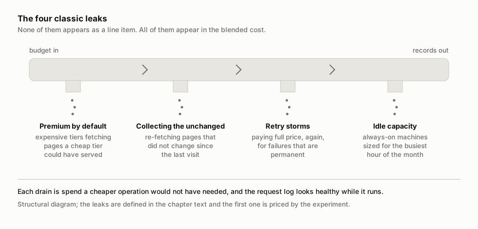
Premium by default is the expensive one, and the experiment has already priced it. Run the premium method first and your cost pins to within a quarter of a cent of premium-only, whatever else you built. In operations this leak rarely looks like a decision. A team adopts a rendering browser or an unblocker product for the hard cases, discovers it always works, and routes everything through it, because reliability feels like a virtue. Chapter 3 called this the browser's gravitational pull. The unit math above is what surrendering to it costs.

Collecting the unchanged is subtler. A daily collector happily re-fetches pages whose content has not moved since yesterday, paying full collection price to learn nothing. The remedy is change detection, any cheap signal that a page changed since your last visit, such as a listing's own updated timestamp or a sitemap date the source already publishes, consulted before the full fetch is paid for. It pairs with the raw-response cache Chapter 7 made the default: never re-buy a page your own storage already holds. In slow-moving catalogs, and most catalogs move slower than their collectors do, this is the largest single discount available. I say that as operator judgment, because how much of your catalog changes per day is a number only your own data can give you.

Retry storms are Chapter 6's lesson arriving as a bill. That chapter split failures into ambiguous ones, worth retrying with growing pauses, and definitive ones, where the source has already answered. A retry against a permanent failure buys the same answer again at full price, as many times as the policy allows, and a fleet doing this on a bad night multiplies its own cost while delivering nothing new. The fix is to classify the failure before any retry fires, and it costs nothing to build.

Idle capacity is the least glamorous drain. Collection is bursty by nature, nightly jobs and weekly sweeps with quiet stretches between, and a fleet of always-on machines sized for the busiest hour keeps billing through the empty ones as well. Compute that scales to zero between jobs fits this workload unusually well. This one is operator judgment rather than a measured result, but of the four leaks it is the one your cloud invoice will confirm fastest.

Cost observability

None of the measured rates in this chapter exist anywhere except inside an operation that records them. The 63.8% and the 93.4% belong to the mid and premium methods meeting your leftovers, and no vendor can print your leftovers in a brochure. So the instrument that makes cost engineering possible is embarrassingly small: tag every attempt with its method, its unit price, and its outcome, and keep Chapter 3's habit of writing which door served each record into the record itself. From those tags, the per-tier rates inside your funnel and the true blended cost fall out as queries instead of modeling exercises. That is the rule underneath this chapter: measure the blended number rather than modeling it, because the modeled one ran 25% under the measured one in a world where every input stayed true.

Pricing from the measured cost

Sooner or later the unit cost has to face a customer, and the order of operations matters. Price from the measured cost instead of the modeled one; a contract priced against the naive $0.01454 gives away $3,565 a month of imagined margin before anything has even gone wrong. Put the delivery floor into the contract next to the price, because a unit price without a coverage promise invites the cream-skimming trap from the run, and a buyer who has read this chapter will ask for both numbers.

Build the margin against the bound rather than the sunny day. Sources change, and Chapter 10 was about how they change without telling you. When a source hardens, its items get harder, which in this model's terms is correlation rising, and your blended cost drifts up the way the chart's waterfall line drifts from $0.01454 toward $0.01990. A price with margin at the sunny-day cost and none at the bound is a price that a single source redesign turns into a loss. The bound is knowable in advance. Price above it, and a hard month re-prices your funnel without re-opening your contract. The tags from the last section then finish the job: when the cheap tier's share starts sliding, you see the migration and its cost the week it begins, long before the invoice does.

Sit in the buyer's chair for a moment. Chapter 1 made you collect three quotes on one specification, and its model prices the spread you should expect: half of list to double it. This model shows where such spreads come from: two vendors selling identical records can sit 2.82x apart on cost purely from routing order. So the spread comes from routing, a low quote is not automatically corner-cutting, and a seller should put both numbers in writing before a buyer has to ask. A low price with no floor is the $0.00250 trap from the table, the one that delivered 40% of the items.

Every division in this chapter had the same denominator, records successfully delivered, and I have been treating that word, delivered, as solid ground, as if an operation always knows which rows reached the customer. It is time to admit that it often does not. Pipelines mark records delivered because an upload call returned. Status fields drift away from what the customer's storage actually holds. A bill computed on this chapter's arithmetic is only as good as the count underneath it. That count is won or lost at the destination, in the customer's own storage.