The Data Collection Handbook · Part III. Trusting the Data

Chapter 10. Monitoring, Drift, and Healing

David Martin Riveros · Published August 7, 2026

A source I collected for years redesigned its product pages on a Tuesday. I found out the following Tuesday, from the customer. For seven days the collector had run every night without a hiccup. Every request came back 200. Every job finished. Every dashboard was green. And every night it had delivered a catalog of products with no prices, because the price now lived in a node my selector no longer matched, and the code, finding nothing, wrote nothing. Seven days of clean, complete, on-time deliveries of garbage. Nothing had broken in any way my monitoring could see, because I was monitoring the pipe and the data was rotting inside it.

That week taught me the last lesson of Part III. You can collect honestly, prove each row correct, and estimate how much you have, and still wake up shipping wrong data, because a source changed under you and told no one. Every source will. This chapter is about catching that from the data itself, fast, before a customer does, and it starts by admitting that the dashboards you already have are looking in the wrong place.

Three failure surfaces

A collector fails on three distinct surfaces, often separately and sometimes stacked, and each is blind to the monitors built for the other two. Keep them separate, because the fix for each is different.

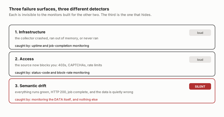
The first is infrastructure. The program crashed, ran out of memory, threw an exception, or, the sneakiest version, never started because a schedule quietly failed. This surface is loud and well served by ordinary monitoring: an exit code, a missing heartbeat, a job that did not complete.

The second is access. The source started refusing you, with a spike of 403s or rate-limit responses, a challenge page, a redirect to a sign-in wall, or a sudden collapse in response size as a real page turns into a short error. Also loud, if you watch for it: status codes and block rates catch it.

The third is semantic drift, and it is the one that ended my week. The program is healthy, so infrastructure monitoring is green. The source served a real page with a 200, so access monitoring is green. The job extracted its rows and finished. And the data is wrong, because the page changed shape and the parser is now reading the wrong thing or nothing at all. No infrastructure or access monitor can see this, because both watch the transport and the transport worked perfectly. Only a monitor that looks at the content can catch it, which is exactly the monitor most teams never build.

Why the green dashboard lies

The reason is structural, not a shortcoming you fix with a nicer dashboard. Every standard operational metric, uptime, latency, error rate, status mix, queue depth, is computed on the pipe: did the request go out, did a response come back, how fast, with what code. None of them is computed on the meaning of what came back. A request that succeeds and returns a page whose price field is empty is, to every transport metric, a complete success. The dashboard is not broken. It is answering a different question than the one you care about, and answering it correctly.

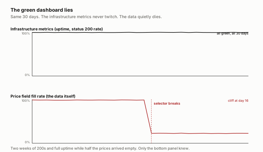
So the rule is simple and most operations violate it: monitor the data, not just the pipe. A green transport dashboard is never evidence of good data. Treat data quality as its own surface, watched by its own signals, or you are watching a smoke detector wired to the wrong room.

Signals from the data itself

The good news is that the data-quality signals are cheap, and you met the most important one in Chapter 8. Per-field fill rate, the share of rows where a field arrived with a real value, is one counter per field per run and the single most useful drift detector there is. My Tuesday break would have shown as the price fill rate falling off a cliff, on the day it happened.

But fill rate has a blind spot that is the most dangerous false comfort in this whole subject, so never read a full fill rate as health. A large class of breaks keeps a field 100 percent populated while its meaning silently changes. A site starts emitting prices in cents instead of dollars and a median of 49.99 becomes 4999. A locale flips and the parser reads a European 1.299,00 as 1.299. A rating field quietly collapses to a default and every row reads 0.0. In each case the field is present, non-null, and completely wrong, and fill rate never twitches. This is Chapter 7's silent-wrong failure and Chapter 6's forbidden edge, arriving now as a monitoring problem.

Catching it needs one more signal: watch the distribution of a field's values, not just whether they are present. Store a small fingerprint of each field each run, a handful of quantiles or a histogram binned against a fixed baseline, and compare this run's shape to the baseline's. The cents shift jumps every quantile by a factor of a hundred. The collapse-to-default drops the field's variety to a single value. A standard tool for the comparison is the population stability index. It scores how far this run's distribution has moved from the baseline's, weighting each bin's change by the log of its ratio. A rough convention: below 0.10 is noise, 0.10 to 0.25 is worth investigating, above 0.25 is a real shift to act on. Reach for a library that computes it rather than hand-rolling a plain distance. Those thresholds are calibrated to that specific weighting, and the index misbehaves when a baseline bin is nearly empty or a new value lands outside every baseline bin, cases a good implementation guards against and a quick one does not. One caution that saves you from a monitor nobody trusts: do not alarm on the p-value of a statistical test. At scraping volumes any tiny difference is statistically significant, so a p-value alarm fires constantly. Alarm on the size of the shift, not on whether a test could detect it.

Two more disciplines make these signals trustworthy. Watch them per segment, never only in aggregate, because a run with the right total row count can hide one category that collapsed while another grew: a high-volume category holding steady masks a low-volume one whose page template broke and whose fill rate went to zero, and the blended number never twitches. And build baselines from statistics that shrug off a bad day, a median and a scaled median absolute deviation rather than a mean and a standard deviation, because a single bad run poisons a mean-based baseline and then either mutes real alarms or floods you with false ones afterward. Scale the median absolute deviation by about 1.48 to make it stand in for a standard deviation, or the limits come out half as wide as they should and the alarms flood.

Alert design

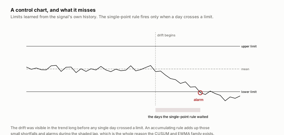
Once you have a signal, you have to decide when it fires, and this is where most monitoring is quietly bad. The naive choice is a fixed threshold: alarm when the fill rate drops below some line. It is either too jumpy, set close enough to catch small problems that normal noise trips it, or too slow, set far enough out to avoid false alarms that a real degradation has to become severe before it crosses. A history-aware rule does better by learning the signal's normal wobble from its own past, which is the control chart: alarm when a day falls more than a few standard deviations below the baseline the signal itself established.

But even the control chart has a weakness, and it is exactly the weakness that matters most for scraping. The basic control chart judges one point at a time against its limits, so it is built to catch a sudden jump. A slow drift, a redesign rolling out to more pages each day, moves the signal down in steps too small for any single day to cross a limit, and the one-point rule waits, and waits, until the drift is finally large enough. The whole family of accumulating rules exists for this case. A rule like CUSUM keeps a running sum of each day's small shortfall below normal, floored at zero so a good stretch cannot bank credit against a future break, and fires when the sum builds up, so it catches a consistent gentle drift while every individual day still looks fine.

This chapter's experiment measures the trade. It simulates 150 days of a field's fill rate, injects a gradual break that drifts the rate down by a total of about twice the daily noise, spread over 25 days, and runs three rules over it: a fixed threshold, a control chart, and an accumulating CUSUM. The only fair comparison is at a matched false-alarm budget, so the code tunes each rule to the same rate of false alarms and then measures how fast each one catches the real break, across hundreds of trials. Everything is offline and seeded, so python run.py reproduces it.

One thing the experiment holds fixed is worth saying out loud before the numbers, because it decides whether any of this survives contact with a real deployment: the budget is per signal. The run tunes one signal to one false alarm a year. Watch every field across every segment with two rules each and you are running hundreds of signals, and a per-signal budget of one false alarm a year becomes a page every few days across the fleet. The alarm you carefully tuned is drowned by the arithmetic of how many you are running. A real deployment needs a budget for the whole system, not each signal: group related fields, page only on the few that carry the delivery, and let the rest raise a quiet ticket instead of a phone call. Otherwise the most sensitive monitor in the world just trains the team to silence it.

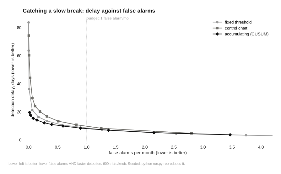
At a loose budget of one false alarm a month, the three rules are close: the accumulating rule catches the break in 8 days against 11 for the control chart. That gap looks small, and it is where the story would end if you monitored the way demos do. But no real on-call rotation wants a false page every month. Tighten the budget to roughly one false alarm a year, the rate a team actually tolerates, and the rules pull apart. The accumulating rule still catches the break in 15 days and catches every break. The control chart now takes 30 days and misses about one break in twenty-five entirely. The frontier chart shows why: as you demand fewer false alarms, the single-point rules' detection delay climbs steeply, while the accumulating rule barely moves. For a slow drift, at the budgets real operations run, the accumulating rule is not a little better. It is the difference between catching the break and not.

Two notes, because the experiment has edges. The advantage is specific to slow, small drifts. As a rule of thumb from process control, once a shift is both large and abrupt, a cliff of two sigma or more in a single step, a plain one-point control chart catches the sudden drop as fast or faster, because one day is already extreme. The practical answer is to run both: an accumulating rule for the slow creep and a one-point rule for the cliff. And in this test the fixed threshold looked competitive, even beating the control chart at the strict budget, but only because the baseline sat still and I placed the line at the right level. On a real signal whose normal level trends, or swings with a weekly cycle, a fixed line is either too jumpy or too slow, and learning the normal from history is the control chart's entire reason to exist. The durable lesson is not which rule to worship, but that choosing the alarm is a statistics question, and monitoring quality lives or dies there, not on how the dashboard looks.

Baselines, and the trap inside them

Every rule above rests on a baseline, so two things about baselines decide whether any of it works. First, never alarm without one, and give it long enough to learn the signal's real rhythm. A field with a weekly cycle needs a baseline that handles the cycle, either spanning several weeks, or comparing each day only to the same weekday, or watching the difference from seven days earlier so the weekly swing cancels out. Skip that and the rule cries wolf every weekend, the team tunes it out, and you have bought alert fatigue, which is worse than no alarm at all because now a real one gets ignored too.

Second, and this is the subtle one, beware the baseline that quietly absorbs the thing you are trying to catch. If your rule always compares today against a trailing window of recent history, then a slow degradation becomes part of the history it is compared to. Each day looks normal against a yesterday that was already a little broken, and the drift walks the baseline down with it, and no alarm ever fires. The break you most need to catch, the gradual one, is exactly the break a rolling baseline hides. The defense is to anchor the baseline to a known-good period rather than a floating recent window, and to re-anchor it deliberately after a verified change, never automatically.

The healing loop

Detection is only worth what you do with it, and a break should run through the same loop every time. Detect it, from the data signal. Diagnose it, starting with which of the three surfaces failed, because the response is different for each: restart the box for infrastructure, rotate identity or back off for access, repair the parser for semantic drift. Fix it. Then verify the fix with the same monitor that caught the break, so you know the signal came back, not just that you changed some code. And last, leave a regression sentinel behind: a check that this exact break, this field going empty or this distribution shifting, would fire immediately if it ever returned. A break you fixed without a sentinel is a break that can come back silently, and the second time is always more expensive.

There is a fashionable idea that this loop can be automated end to end, a collector that detects its own drift and re-derives the broken selector without a human. Some of that is real and useful, especially the detection and the fallback to a second extraction method. But treat automatic repair with suspicion, because an auto-fix that makes the signal look healthy again can just as easily be papering over a deeper change with a plausible wrong answer, which is the exact failure this whole book warns against, now dressed as a feature: the pipeline reports success while shipping data that is quietly wrong. Automate the detection freely. Put a human at the gate of the fix.

What monitoring actually buys

Be honest about the promise, because it is easy to oversell. Monitoring does not stop sources from changing. It does not prevent breaks. What it does is bound how long you stay ignorant of one, and that bound is the whole game. A data operation runs on two clocks: the time to detect a problem and the time to recover from it. For many collector breaks recovery is the shorter clock, because once you know, a selector swap or a parser fix is quick, though a hardened block or a full schema redesign can drag it out. Detection is the clock you control least by default, because without a data signal you do not learn about a silent break until it has shipped for days and a customer has already made decisions on it. The cost of an error climbs steeply the longer it goes unseen, from cheap to catch at the moment it enters, to costly to correct once it is in the data, to ruinous once someone downstream has acted on it. Be precise about how much monitoring buys, because the chapter's own experiment sets the ceiling: a hard cliff that empties a field moves detection to about a day, but the slow drift the chapter spends most of its ink on still takes on the order of two weeks to catch even with the best rule. That is not a small win. Two weeks beats the alternative, which is a customer telling you a month later, and moving detection from a month to a fortnight is the largest lever you have on the total cost of being wrong.

Which is the close of Part III. You can collect it, trust it, size it, and watch it, and all of that is engineering you now know how to do. What none of it has asked yet is what the whole thing costs to run, and whether the economics work at the scale a real customer needs. That is the subject of Part IV, and it starts with the one number that decides whether a collection business lives or dies: the cost of a single delivered record.