The Data Collection Handbook · Part III. Trusting the Data

Chapter 9. Coverage: Collecting Everything

David Martin Riveros · Published August 6, 2026

Every chapter until now has been about the rows you collected: getting them honestly, getting them right, proving they are correct. This chapter is about the rows you did not collect, and it is harder, because a missing row leaves no trace. A wrong price sits in the data where you can find it and argue with it. A product that was never collected is simply absent, and absence is invisible. No validator from the last chapter can flag a row that is not there. The file looks complete. The schema passes. The counts look big. And a third of the catalog is quietly gone.

That is the shape of the worst coverage failures: they are success-shaped. The scrape finished, every request returned a normal response, the row count looked healthy, and nobody saw the hole. This chapter is about the one question that hole hides behind, the hardest question in the field, "did we get all of it?", and how to answer it with a method and an estimate instead of a shrug.

Where rows go missing

Rows do not usually vanish dramatically. They leak, and four failure modes account for most of the leak, all sharing one property: the collector terminates cleanly and reports success while missing data. There is a fifth that hides even better, a scope quietly narrowed before you began, a default filter or a region setting that shrank the universe you thought you were collecting, and the coverage contract later in this chapter is where you pin the scope down so that one cannot bite. Learn to see the four, because your monitoring will not.

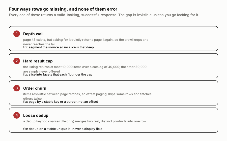
The first is the depth wall. A site serves the first several pages normally and then quietly stops: ask for page 43 and it hands back page 1 again, or an empty page, or the last page it is willing to serve. Your crawler, paging happily, loops or halts and never reaches the tail, and every one of those requests returned a valid page. The fix is to never trust a page count you were given, and to probe the wall on purpose, one careful request a little past where you expect the end, checking whether its contents are actually new. Probe gently: a request for page one million forces the source to scan its whole index, which is neither fair load nor a good way to stay unblocked.

The second is the hard result cap, and it is so common it is nearly a law of the web. A listing announces a million results and the backend will only ever hand out the first N, almost always a round number. The reason is concrete and worth knowing. The default result window in Elasticsearch, the search engine behind a great many storefronts, is exactly 10,000, so deep pagination past the ten-thousandth result is refused outright, and many deployments also stop reporting an exact total past that window, which is why "10,000+" is so common a sight. Other backends draw the line elsewhere and just as hard. eBay's finding interface caps at 100 results per page and 100 pages, exactly 10,000 per query. The GitHub search interface stops at 1,000. A common maps interface returns at most 60 places per query, however many thousands exist. If the number of rows a query actually returned lands on a suspiciously round number, that is almost never the size of the catalog. It is the cap.

The third is order churn. If items reshuffle between your page fetches, and on a busy catalog they do, then paging by position skips some rows and fetches others twice. The duplicate rate is your only visible symptom, which is why duplicates are worth watching rather than silently discarding. The fix is to page by a stable key or a cursor rather than a numeric offset. When the site offers only page numbers, buy back the same safety by overlapping your pages, striding less than a page at a time, and deduping the overlap on a stable key.

The fourth hides inside a habit that feels like hygiene: deduplication. A dedup key that is too loose, matching on a display title rather than a stable identifier, quietly merges two genuinely distinct products into one row and calls it cleaning. The drop counter reads like tidiness and is actually a coverage-loss counter. Dedup on a real unique identifier, never on a field a human reads.

Segmentation: slicing under the cap

The cap is the killer you beat with arithmetic, and the tool is segmentation: if the whole catalog will not come through one query, slice it into facets that each fit. Category, brand, price band, geography, date; any attribute that partitions the catalog into pieces small enough to clear the ceiling.

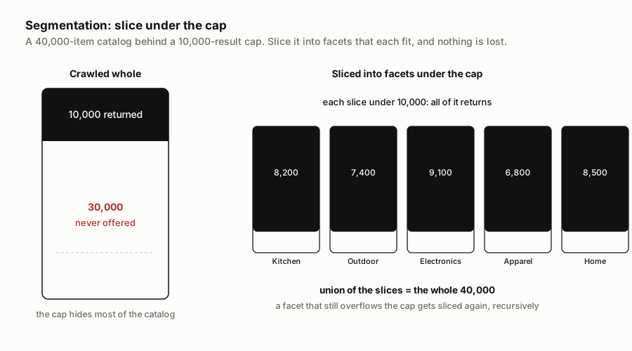
Picture a catalog of 40,000 items behind a 10,000 cap. Crawl it whole and you get 10,000, with 30,000 you never even knew to miss. Read the site's own category counts first, slice into facets each under 10,000, collect each in full, and stitch them back together on a stable identity key. The union is the whole catalog only if the facets actually cover it, so check that rather than assume it: real category systems let an item live in two facets or none, so compare the distinct keys in your union against an independent count before you believe you are whole. Two disciplines make the slicing trustworthy. When a facet is itself over the cap, split it again, halving a price or date range until every piece fits. That terminates as long as no single value on the axis holds more than the cap; when a pile of items shares one price or one brand with nothing left to bisect, switch to a different axis or accept a residual over-cap slice and flag it as incomplete. And treat any slice that returns exactly the cap as unresolved rather than finished: a count that lands precisely on the ceiling is a truncation warning to subdivide or verify, not a total to book, however plausible the page makes it look.

Counting what you cannot see

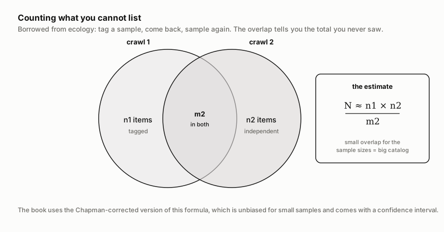
Segmentation gets you more of the catalog. It does not tell you how much you are still missing, and for that you need to estimate a total you can never enumerate. The method is borrowed, beautifully, from ecology. To count fish in a lake you cannot drain, you net a sample, tag them, throw them back, come another day and net a second sample. The fraction of the second catch that carries a tag tells you how big the lake's population must be: if few of your tagged fish come back, the lake is large; if most do, it is small. Catalogs make this easier than lakes, because you never have to tag anything. Every item already wears a stable identifier, a product code or a canonical link, so you crawl the catalog twice by independent routes, record the identifiers each pass saw, and the items that turn up in both passes are your recaptured tags.

This is not a toy. The United States grades its own census this way. After the 2020 count, the Census Bureau ran a second, independent survey and used the same two-sample overlap idea, dual-system estimation, to measure how good the count had been. The stakes are why it bothers: on the order of a trillion dollars a year in federal funding rides on census numbers, so knowing how far off they are is worth a great deal. Decades earlier, two researchers estimated the size of the entire indexable web the same way, by measuring how much different search engines' results overlapped, and put a floor under it of 320 million pages. The method that counts fish, and people, and the web, will count a product catalog.

The estimator this chapter uses is the Lincoln-Petersen formula with a small-sample correction, the Chapman estimator, which removes nearly all the bias the raw version carries, and it comes with a confidence interval so the answer arrives knowing how firm it is. Two assumptions ride under it and both matter for catalogs. The catalog must hold still between the two crawls, so run them close together, ideally the same day, or the estimate lands on whatever size the catalog was at the second pass. And the method can only ever size the part of the catalog your two routes could reach; items no route can touch, gated behind a login, bound to a region, linked from nowhere, sit outside the number entirely. The example puts the estimator to the test on a synthetic catalog whose true size is known only to the grader, with each crawl drawing genuinely at random, so every estimate can be marked right or wrong.

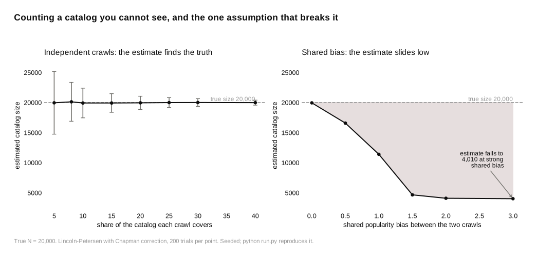
The good news first, on a simulated catalog of 20,000 items with each crawl drawing at random. Two independent crawls covering just a fifth each estimate its size well. Repeat the experiment many times and the estimates average within a third of a percent of the truth, so the estimator carries almost no bias. Any single pair of crawls is looser than that, and candid about it: the 95 percent interval is about plus or minus 5.5 percent, and it contains the truth 94 percent of the time, close to the 95 it promises. Even at a fifth each you can bound a catalog you never saw whole, and the interval tells you how tightly. Crawl more and it shrinks; at 40 percent each the interval is down to about 2 percent. The estimate is trustworthy, and it knows how trustworthy it is.

Then the run breaks it on purpose, because the method rests on a third assumption that catalog crawling loves to violate: the two crawls must be independent. In the experiment both crawls are given the same popularity bias, favoring the same easy-to-reach items, which is exactly what happens when you crawl the same relevance-sorted list twice or route both crawls through the same discovery path. Independence is gone, and the damage is severe. Both crawls keep finding the same popular items, so the overlap inflates, and an inflated overlap says the catalog is small. At a strong shared bias the estimate collapses from 20,000 to about 4,000, an 80 percent underestimate, and its confidence interval now contains the truth zero percent of the time. That last number is the one to sit with. The estimate is not just wrong, it is confidently wrong, reporting a tight interval around a number that is nowhere near right. The reason is that the overlap sits in the denominator of both the estimate and the interval, so a fat overlap pulls the estimate down and pulls the interval tight at the same moment. The math did not fail. The independence assumption did, and the interval had no way to know.

Follow that underestimate one step further, because its business meaning is the trap. If the method says the catalog is smaller than it is, then the haul you actually collected looks like a larger share of it than it is, and your coverage number comes out flattering. Worse, this is the common direction on the open web, not a rare accident. Search rank, sitemap freshness, category placement, and internal links all favor the same popular head items, so any two crawls that lean on the site's own structure lean the same way and quietly agree to overstate how complete you are. The comfortable error and the dangerous error are the same error.

There is a cheap check for this, and it costs one line of arithmetic. Under true independence the overlap should land near n1 times n2 divided by the catalog size. Take a rough size you trust to be roughly right or a little low, and compare. If the overlap you observed is well above what that predicts, say half again or more, then either your two crawls are correlated or the true catalog is far smaller than your rough figure, and both readings forbid trusting the estimate. An overlap far below the prediction is its own warning, of crawls that repel each other and overstate the catalog. Run the check, in both directions, before you believe any capture-recapture number.

So the practical rule the experiment points to is that the two crawls must reach the catalog by genuinely different routes. Different discovery mechanisms above all, one by category walk and one by sitemap or a public interface, then different sort orders and segmentation axes, enough that the items one crawl finds easily are not the same items the other finds easily. Two crawls that share a proxy pool, a login, a geography, or a discovery path share their blind spots, and shared blind spots are what quietly turn this estimator into a confident lie. Different routes reduce the bias; they do not abolish it, because items that are hard for everyone to reach stay hard for both crawls, so treat the corrected number as a lower bound on the catalog, not a fact. And re-running the same crawler a week later is not a second sample. It is a reliability test wearing a coverage estimate's clothes, and it will report near-total overlap and tell you that you have everything.

The second pass can also be small, which matters because this book never stops caring about fair load. It does not have to be a whole second crawl; a modest independent probe carries enough overlap to size the catalog, as long as the overlap is actually there. Size the probe from the arithmetic before you run it, since expected overlap is n1 times n2 over the catalog size, and if that lands in single digits the estimate will be noise. For a fixed request budget the tightest interval comes from two equal passes, so if grading coverage is the goal, split the budget in half. If collecting the most items is the goal instead, a large main crawl and a small probe gather more of the catalog while still buying a rough bound, and that is a real choice, not an oversight.

Keep the division of labor straight, because the two techniques in this chapter answer different halves of the question. Segmentation locates items, pulling more of the catalog through the caps, but it can never tell you when you are done. Capture-recapture sizes the gap, telling you what fraction is still missing, but it never tells you which items those are, and it sizes only the catalog your two routes could reach. Segmentation to collect, capture-recapture to grade the collection: that pair, together, is the best answer to "did we get all of it."

Coverage in production

A single estimate answers "did we get it all today." Production needs a standing answer, because coverage rots on its own: sites restructure, caps change, a category stops rendering, and a slice goes dark between one delivery and the next with nothing in the logs. Three cheap habits keep the answer current.

Reconcile distinct keys, not raw rows, against the site's own claimed counts, and test for a stable ratio rather than equality. Raw row counts lie in both directions, rising on duplicate pagination while true coverage falls; distinct identifiers do not. And the site's number is itself a second noisy measurement, capped and rounded and sometimes personalized, so the accurate statement is never "we match the site" but "our count and the site's sit in their usual ratio." A ratio that suddenly moves is the alarm. A third independent number sharpens it: a site's sitemap files, capped by protocol at fifty thousand URLs each, give a count that neither the listing pages nor your crawl produced, and three numbers that usually agree catch a problem two never would.

Plant sentinels: a fixed panel of known items that must appear every run, so their disappearance is a coverage alarm you do not have to compute. The power is worth knowing exactly, limits and all. A panel of 50 sentinels catches a uniform 5 percent loss about 92 percent of the time in a single run. A 1 percent loss it catches only about 40 percent of the time in one run, though that climbs toward 92 percent across five runs. Two conditions hide in those numbers. They assume the loss is spread evenly, and it rarely is, so a panel scattered at random can hold nothing from the one category that broke; weight the panel toward the segments you most need to be sure of. And the five-run climb assumes the loss reshuffles run to run, as flaky fetches do; a permanent structural gap either sits in a sentinel from the first run or never will, so it shows immediately or not at all. Sentinels are smoke detectors. They catch a real fire cheaply, and they promise nothing about the corners.

Watch coverage per segment, not just in total, because the total is the weakest signal you have and the one most teams rely on. Losses are almost never spread evenly; they concentrate in the corner that broke, one category, one region, the newest and fastest-changing items, which are usually the commercially valuable ones. I have shipped a feed that came in two percent light overall, comfortably inside the band, while one whole category had silently dropped by forty percent. The invoice said complete, the customer priced their own decisions on the delivery, and the missing forty percent surfaced weeks later not as a scraper bug but as a wrong business call someone had already made on it. The total hid the gap. A per-segment view shows it at a glance, and it is the difference between finding the hole yourself and having a customer find it for you.

One caution the production numbers teach, because it cuts the other way. A big overnight drop is not always your bug. Real catalogs do cliff: in 2016 a well-known supermarket pulled a major supplier's brands from its site overnight in a pricing dispute, and dozens of brands vanished at once. A collector that cried failure that morning would have been wrong; the site really had changed. And a drop of a few dozen items in a feed of forty thousand is a rounding error against the total while being a total wipeout of that one supplier's segment, which is the whole case for watching segments rather than the sum. Coverage monitoring has to tell a collection regression from a real catalog change, which is exactly why you reconcile against the source instead of only against yesterday.

The coverage contract

All of this rolls up into how you state coverage to whoever pays for the data, and the standard is higher than the industry usually meets. Do not say "we scraped the whole site." That is a claim with no method behind it, and a claim with no method is a hope. State four things instead. The scope: exactly which universe you set out to collect. The method: how you collected it and how you segmented to beat the caps. The two independent routes you crawled, with the result of the overlap check, so the estimate's own assumption sits on the record. And an estimated completeness with its basis. For a category that might read: an estimated 96 percent, by two-sample capture-recapture over a category walk and a sitemap, 95 percent interval 94 to 98 percent. That is a number a buyer can weigh, and a number a serious buyer will ask for. The buyer's move is to write it into the agreement as a term, not a courtesy: a completeness floor, a cadence for re-measuring it, and a remedy when it slips.

Two riders belong in that contract, and both come straight from the experiment and the research behind it. First, a completeness percentage is a population estimate, never a promise about any one item; 96 percent coverage is fully compatible with missing the single product a buyer cares most about, so an aggregate number and a spot-check of the items that matter are different assurances and a buyer should want both. The census makes the point at national scale: its 2020 net national miss was about a quarter of a percent, not even distinguishable from zero, while one major demographic group was undercounted by nearly five percent. A blended figure can hide a segment gap large enough to matter, which is why coverage is always reported per segment, never as one comforting number. Second, coverage estimates expire. A figure measured at onboarding and never rechecked is a stale claim the day a site restructures, so tie the re-measurement to the commercial rhythm the reader already has: every delivery or billing cycle ships with a coverage number dated inside that cycle, and a number that stops moving is a number nobody is checking.

The buyer's side of this is a single question that separates a real data operation from a hopeful one. Not "how many rows," but "how do you know that is all of them, and what is your estimated coverage with its interval." Volume without a denominator says nothing. Ten million records is a big number attached to an unknown fraction, and a smaller dataset with a measured 97 percent is worth more for any use that leans on the catalog being representative, which is most uses worth paying for. That measured denominator also changes how a buyer shops. It turns a vendor comparison from price per row, which rewards padding, into price per percent of the universe covered, which rewards the thing you actually want. Watch the scope line while you do it, because a coverage percentage is trivially inflated by quietly shrinking the universe it is measured against. The number that means anything is completeness against the scope you were promised, not against whatever was easy to reach. A row count is not coverage. Coverage is a fraction, and the professional move is to estimate the denominator instead of pretending it does not exist.

You now have data you can trust to be correct, and a way to know how much of it you have. The last thing that can go wrong is that it was all true when you checked and quietly stopped being true afterward, because a source changes without telling you. Catching that, from the data itself, before a customer does, is the subject of Chapter 10.